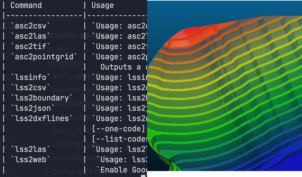

In an attempt to go back to basics and improve knowledge of file handling in C, I have developed a simple set of CLI tools for working primarily with .asc raster files.
This developed on to working with .00X files. These are 'load files' used by the software LSS which is heavily used in the British quarrying industry and surveying.
The result piece of software is capable of converting thesse two file types into frequently used products by myself and others within the indsutry.
The intention was to improve my knowledge of C and create a minimal set of scripts for converting without any dependencies to keep them as light-weight as possible.
I decided that I first wanted to work with .asc raster files. I have spent a lot of time playing around with pointcloud and 3d datasets, and so a fast way to convert these 2D files with 3D information was something that would prove useful.
The ascii format is well documented and also allowed for easy reading of the files in text editors such as VSCode to check the layout. This made it the perfect starting point for developing on C knowledge in a geospatial setting.
The first step was to just be able to load a file using C and print statistical information about it. Luckily the ascii files header contains most of the required information for this.
From this my first plan was to convert .asc files to .csv with XYZ which could then be loaded into software such as CloudCompare as a pointcloud. So the header gives us the size of each entry (CELLSIZE), the number of rows in the file and cells per row (NROWS, NCOLS). We can use XLLCORNER and YLLCORNER to get the lower left corner of the file, and use XLLCORNER + (CELLSIZE * NCOLS) and YLLCORNER + (CELLSIZE * NROWS) to then get the top right corner of the file. The following rows are then each cell of this bounding box, starting from the top left of the image. In order to implement the csv generation from ascii files, the code needs to read the file and extract all data entries where the value does not equal the NODATA value. This makes the generation of the csv simple.

The next task was converting the ascii file to a .las pointcloud file. Luckily this format is also well documented.
My previous workflow would have been to convert the pixels to points in QGIS, export a csv of the results and then import into CloudCompare where it is possible to save as a las.
There were 2 issues with this. The first is the fact that using GIS took multiple steps. This could be simplified into a model workflow using QGIS model builder which was my old preferred method, however to have an almost instant conversion feels much more satisfying.
The other issue is that the cloud is purely XYZ. It is possible to colour by height-ramp in CloudCompare, however, I wanted to include an argument for generating a viridis RGB value for each point colour-ramped off of the min and max Z values.
The generation of the las only required the writing of the headers, where values were updated based on simple calculations such as the max X,Y,Z values. Then the points were added, again with NODATA values being excluded from the pointcloud.
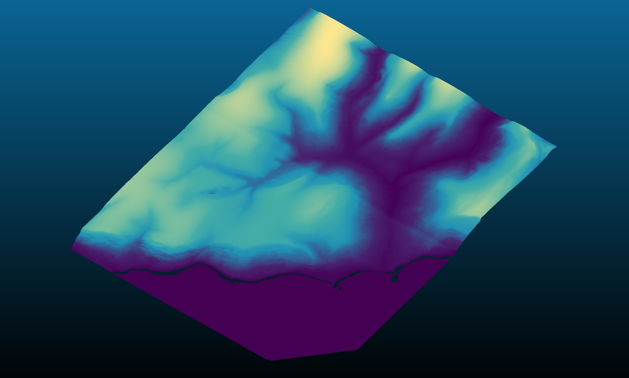
The result is a fast conversion of points directly written into a .las file which can then be used in various software for 3d visualisation.
The next tool is asc2pointgrid which generates a .dxf file of blocks in the appearance of crosses on a given spacing by the user.
Once again, the format of the .dxf file is documented online or can be viewed by opening the file within a text editor. For this example, I made a simple dxf file using AutoCAD with a block at 0,0 of a cross with a Z value of 15. Afterwards, I inspected the file within VsCode where I could understand how it worked.
From this, all that had to be done was to tweek the csv generating code to write out the dxf format and generate the block at our given positions as well as assigning the Z value as a property.
As well as this a small text item is inserted slightly offset from the block with the Z value of that point.

This tool was developed to provide quick spot level drawings from an ascii grid that may be exported from a number of packages. The dxf is then able to be used it producing final drawings in CAD in an easier manner, or imported into GIS software packages.
The LSS load files store information that is used to load the data into survey files. This is stored as plain text in files ending with extension .001, .002 etc.
The plain text allowed us to read and become familiar with the format of these for future parsing through ASCTools. A few dummy surveys were set up with specific information to look for.
The files contain rows of data like this:
lss_identifier, id, x, y, z, reference
21, 338, 123, 456, 789, .BRK
So as with the las files, the load files contain header information. LSS identifies these with a value of 0. The first step was to ignore rows where the lss_identifier was equal to 0.
The terrain within the file was identified as 21. When checking multiple load files, they always ended with a row containing just the lss_identifier of 9.
This allows us to assume all rows that !=21 can be ignored and now we set up logic for parsing the terrain information.
LSS works using both point and link features. Points can be feature coded, for example as 'PBHOL' which may refer to a borehole. There are also 'non-feature' points which are generally for terrain information.
The link features work slightly differently as they are composed of multiple points. By checking with predefined values and checking the load files this was deduced to use a simple structure too.
The link begins with its reference prefixed with '.'. Following this, every child point of this line did not have the prefix. We can parse subsequent points as being the same line until either the reference changes or we encounter another start of link prefixed with '.'.
Now that the structure is understood, it is possible to begin producing useful conversions of the load files for other pieces of software to use.
First up was a simple conversion to a CSV as the original project was for working with 3D data sets. A CSV files produced the easiest common format for GIS and CloudCompare for producing pointclouds.
This tool simply iterates the terrain data rows, stripping the XYZ values into respective columns using:
lss2csv example.001
Next was a direct conversion to a .las file. With our previous code for reading .asc files, a few simple edits were required before we could then feed the code the point data from the load files.
Using this tool the user can go directly from an LSS survey load file to a .las pointcloud using:
lss2las example.001 [-elev_rgb]
Here the -elev_rgb argument can be used to apply colours to these points using a calculated heightramp of the data.
Next up was converting the link features into polylines for cad or as Linestrings in geojson files. For this the load file is parsed to determine which rows are links and then producing individual lines from these returned rows.
This can be produced using either:
lss2json example.001 or lss2dxf example.001 [--one-code] [--list-codes]
The geojson file will contain all of the link features with a property for their code. The dxf export has the option to only export based on a code. For example, if you only want to find where the crest of faces were this could be done with lss2dxf example.001 --one-code QFL.
The --list-codes option allows for comma delimited feature codes which will be on separate layers. If no argument is given, all codes will be extracted and on separate layers within the dxf file.
Creating a boundary polygon was next up. This tool parses all of the points within the load file and generates a bounding geometry. For this I have chosen geojson as the output with uses the Polygon feature class.
With the code sorted for all of these exports the next to be made was lssinfo which can be used to output:
This information can then be used for a quick overview of the stdout used in performing future tasks. One example could be using the bounding geometry or the centroid to assign the surveys to a master sites polygon database to index surveys by jobs/jobcodes
The final tool was lss2web. This is a tool for producing a quick, shareable .html file containing the survey information.
Using this tool will parse the link features and append them to a Leaflet base map. This is a javascript library for producing quick and simple webmaps.
The lines are appended and coloured using a rough colour dictionary. If feature codes are not in this dictionary, they will default to blue.
By doing this directly into the .html file the output is kept as only 1 file. As long as the recipient or user has an internet connection this map will load and display the information in a visual and interactive way.
LSS2Web can be used with two arguments: -ge and -points. The first adds a Google Satellite imagery basemap below using Google's XYZ tileset. The second argument will include all the points from the survey to be visualised with a z-value derived colour ramp.
Working on ASCTools has been interesting in both understanding lower level lanugages like C as well as having to research file formats to understand their structure and reading non plain text files.
I hope that I can continue to develop new uses for this tool to aid with speeding up workflows and reducing the amount of software for processing between commonly used filetypes.
As previously mentioned, there could be a use in using tools such as the lssinfo in larger scale projects such as producing a database of surveys dependent on location. This would allow an automated service to index the files spatially and then assign associated values such as client, job code, job title etc.
The simplicity of the tools and speed of conversions/data acquisition can allow the ASCTools set to be used as a cog in a much larger machine providing extra quality to other developed systems which I hope to explore in the future.